
General Linear Models
Online lesson from biological data analysis modules

What will you learn?
In this lesson you will learn to:
- Explain the concept of a general linear model
- Describe some examples of general linear models
- Describe the assumptions of a general linear model
- Explain the difference between a response variable and an explanatory variable
Definition
General linear models are a family of statistical models based on the normal distribution.
A lot of classical statistical methods come under the unifying umbrella of general linear models:
- analysis of variance (ANOVA),
- linear regression,
- t-tests,
- analysis of covariance (ANCOVA)
are four examples of statistical methods which are all examples of general linear models.
General linear models are often called linear models for short.
Fitting a General Linear Model
General linear models have parameters, like all statistical models.
Fitting a general linear model means using the data to find suitable values for the parameters of the model.
You can use the lm() function in R to fit a general linear model. Below is an example:
		  # Fit a simple general linear model to the human height data
		  m = lm(HEIGHT ~ 1, data=human)
The lm() function uses a maximum likelihood approach to fit the model, but we don't need to know about the details of the fitting. We will need to know how to interpret the results of the fitting process.
Synonyms
In texts you will see several names used for essentially the same concept. Here are a few that you will encounter in this lesson:
- Error equivalent to residual
- Fitted value equivalent to the prediction from a model
- Explanatory variable equivalent to independent variable or predictor variable
- Response variable equivalent to dependent variable or predicted variable
A statistical glossary on Brightspace has a more complete list of statistical terminology
Example 1
(Video 4 mins 46 sec)
R Code for the above example
lm() command to fit and display the first general linear model shown in the video above.
		  # Subset data for heights of women
		  humanF = subset(human, SEX=='F')

		  # Fit a general linear model to heights of women
		  m = lm(HEIGHT ~ 1, data=humanF)

		  # Produce a summary of the fitted model
		  summary(m)
lm() command to fit and display the second general linear model shown in the video above.
		  # Fit a general linear model to heights of women and men
		  m = lm(HEIGHT ~ 1 + SEX, data=human)

		  # Produce a summary of the fitted model
		  summary(m)
Example 2
Classical linear regression as a general linear model
(Video 3 mins 35 sec)
R Code for the above example
lm() command to fit and display the general linear model shown in the video above.
		  # Subset data for heights of men
		  humanM = subset(human, SEX=='M')

		  # Fit a general linear model to the relationship
		  # between HEIGHT and WEIGHT of men
		  m = lm(HEIGHT ~ 1 + WEIGHT, data=humanM)

		  # Produce a summary of the fitted model
		  summary(m)
Example 3
Classical ANCOVA as a general linear model
(Video 4 mins 4 sec)
R Code for the above example
lm() command to fit and display the general linear model shown in the video above.
		  # Fit a general linear model to the relationship between
		  # height and weight for women and men
		  m = lm(HEIGHT~1+SEX+WEIGHT+SEX:WEIGHT, data=human)

		  # Produce a summary of the fitted model
		  summary(m)
Assumptions
A general linear model makes a number of assumptions about the population it is trying to model.
The main assumptions are (in order of decreasing importance):
- Assumption of independence:
The residuals are independent of one another - Assumption of homogeneity of variance:
The residuals can be described by a single standard deviation.
For linear regression this assumption can be split in two (homogeneity of variance and linearity). - Assumption of normality:
The residuals follow a normal distribution - No uncertainty in explanatory variables:
This assumption is most important for regression type models (e.g. examples 2 and 3 with continuous explanatory variables).
Assumptions (Introduction)
Validating the assumptions of a general linear model
(Video 3 mins 4 sec)
Assumptions (Independence)
Validating the assumptions of a general linear model
(Video 47 secs)
Assumptions (Homogeneity of variance)
Validating the assumptions of a general linear model
(Video 4 mins 41 secs)
Assumptions (Normality)
Validating the assumptions of a general linear model
(Video 1 min)
Assumptions (Overview)
Validating the assumptions of a general linear model
(Video 2 mins 14 sec)
R Code for the above example
lm() command to fit and display the general linear model shown in the video above.
		  # Fit a general linear model to the relationship between
		  # height and weight for women and men
		  m = lm(HEIGHT~1+SEX, data=human)

		  # Produce residuals versus fitted plot (homogeneity of variance)
		  plot(m, which=1)

		  # Produce QQ plot of the residuals (normality)
		  plot(m, which=2)
R will produce four validation plots by default
		  # Display the default four validation plots
		  plot(m)
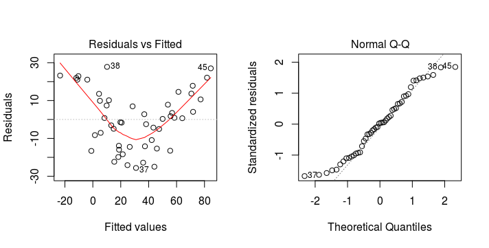
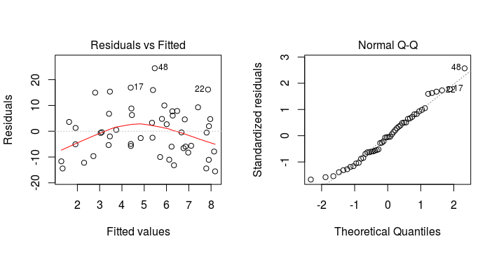
Violation of Assumptions
The assumptions of homogeneity of variance and normality can be validated by looking at the residuals from a fitted general linear model.
General linear models are fairly robust to mild violations of the assumptions. They are most robust to departures from normality.
Below we give some examples of residual versus fitted plots and quantile-quantile plots from fitted general linear models that suggest one of these two assumptions has been violated.
Violation of Normality
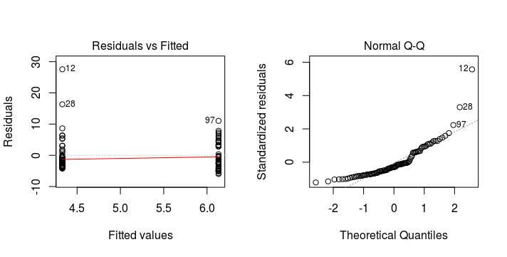
Violation of Normality
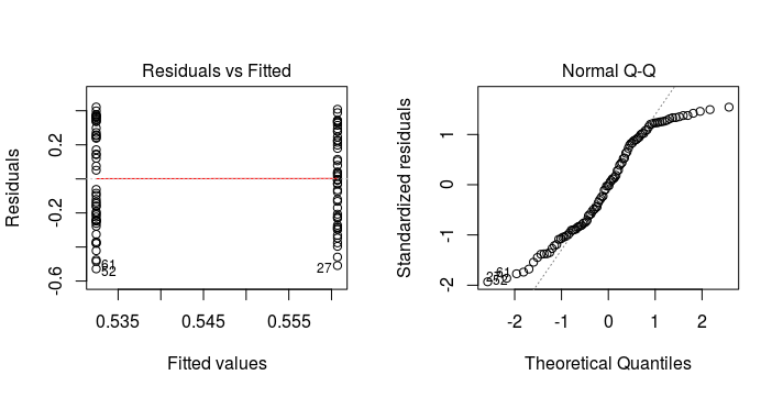
Violation of Homogeneity of Variance
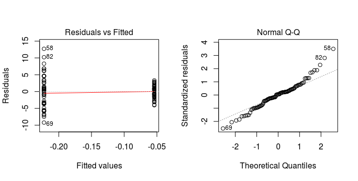
Violation of Homogeneity of Variance
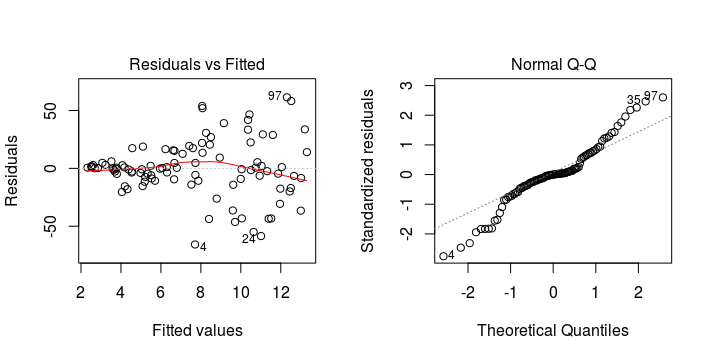
Violation of Homogeneity of Variance
Violation of Homogeneity of Variance
More 'synonyms'
General linear models bring together many classical methods into a single approach. The classical terminology is still used even if the statistical model is a general linear model.
Below are some examples you will come across:
| Classical term | General linear model equivalent |
|---|---|
| ANOVA (analysis of variance) | A general linear model where all explanatory variables (usually no more than two) are qualitative (i.e. factors) |
| t-test | A general linear model with one qualitative explanatory variable with two levels |
| Linear regression | A general linear model with one quantitative continuous explanatory variable, and an expected straight-line relationship between response and explanatory variable |
| ANCOVA (analysis of covariance) | A general linear model with two explanatory variables (one quantitative continuous and one qualitative). |
Key Points
- General linear models are statistical models
- Randomness in the data is always described with a normal distribution
- To be useful the model's assumptions must be valid
- The majority of model assumptions are about the residuals
- Use graphical approaches to test assumptions
- Some model assumptions are best thought of when designing a data collection scheme