
Null-Hypothesis Testing
Online lesson from biological data analysis modules

What will you learn?
In this lesson you will learn to:
- Describe the two common methodologies for null-hypothesis testing
- Define a p-value
- List some limitations of hypothesis testing methodology
Methodology (Part 1)
(Video 3 mins 10 sec)
Methodology (Part 2)
(Video 3 mins 57 sec)
Analogy to a court of law
| H0 Testing | Court of Law | |
|---|---|---|
| Question: | Is H0 false? | Is the defendant guilty? |
| Starting position: | H0 is presumed 'true' | Defendant is presumed innocent until proven guilty |
| Evidence: | Test is based solely upon sample data | Decision of jury based solely upon the presented evidence |
| Errors: False negative | Insufficient evidence to find H0 false | Guilty defendant is found inocent |
| Errors: False positive | H0 is incorrectly found false | An inocent defendant is found guilty |
Methodology Overview
Below is a summary of the two broad methodologies. Fisher's methodology in black and Neyman and Pearson's extension in blue.
- Define a critical significance level (this is commonly taken to be 0.05, and called the alpha level, $\alpha=0.05$).
- Calculate a test statistic (e.g. F-ratio).
- Calculate the p-value
-
Make a black and white decision based on $\alpha$:
- p-value $<\alpha$ we reject H0.
- p-value $\ge \alpha$ then the we fail to reject H0.
An effect is often said to be statistically significant when H0 is rejected.
In the end, the scientist uses the results together with other evidence, and estimated effect sizes, to draw a biological conclusion from the analysis.
R code for null hypothesis testing
		  # Fit models for the hypothesis and the null-hypothesis
		  m1 = lm(HEIGHT~1+SEX, data=human) # Hypothesis model
		  m0 = lm(HEIGHT~1, data=human)     # Null-hypothesis model

		  # Compare these two models
		  anova(m0, m1)
emmeans package.
		  library(emmeans)  # load emmeans package

		  # Estimate effect of SEX on HEIGHT
		  m_effect = emmeans(m1, spec='SEX')

		  # Print effect sizes and 95% confidence intervals
		  confint(m_effect)
Example 1 (Is a dice biased?)
We have already seen this example when discussing statistical modelling.
Question: Is our dice biased?
The two possible answers to this question can be written as hypotheses:
Hypothesis (H1): The dice is biased.
Null-Hypothesis (H0): The dice is unbiased.
Sample Data versus Population
I have a dice that I have rolled 20 times, giving these results:

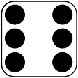


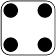
This is a sample of 20 observations from the population.
In this case, the population is an infinite number of rolls of this dice (we will never have complete information about this population).
Step 0: Define a critical significance level
Step 1: Calculate a test statistic
We will use our measure of bias as a test statistic: $$ \text{Bias} = \sum_{i=1}^6 (p_i - 1/6)^2 $$ where $p_i$ is the observed relative frequeny of the ith outcome.
For our data sample:
$p_1=0.3$, $p_2=0.1$, $p_3=0.25$, $p_4=0.1$, $p_5=0.1$, $p_6=0.15$
Giving $$ \text{Bias} = 0.0383 $$
Step 2: Calculate a p-value
What is the probability that a fair dice will give a bias as large as 0.0383? (the answer to this is the p-value)
Below is the distribution of bias from a fair dice (this distribution is calculated from the categorical distribution).
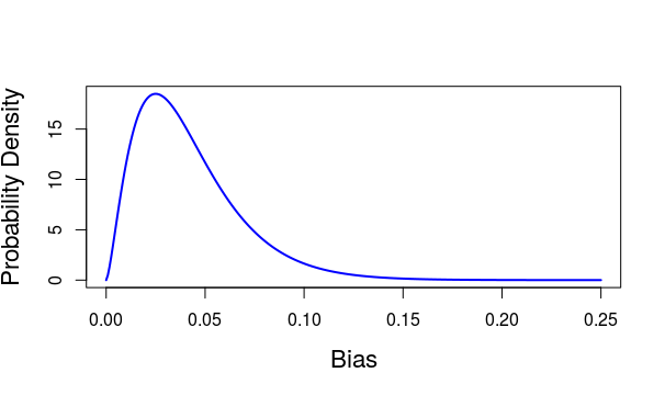
Using this distribution, the p-value is calculated as $$ p = 0.51 $$
Step 3: Make a decision
The p-value (=0.51) is greater than 5%
So we fail to reject our null-hypothesis
We have no evidence from our data that this dice is biased
Example 2 (Human heights)
This is the example discussed in the videos
Question:
Is the average height of adult men diffreent from adult women?
The two possible answers to this question can be written as hypotheses:
Hypothesis (H1): The average height of adult women differs from that of adult men
Null-Hypothesis (H0): The average height of adult women is the same as that of adult men.
Step 0: Define a critical significance level
Step 1: Calculate a test statistic
A general linear model is an appropriate statisical model. So we fit general linear models for the H1 and H0 hypotheses and use an F-ratio as our test statistic.
		  # Fit models for the hypothesis and the null-hypothesis
		  m1 = lm(HEIGHT~1+SEX, data=human) # Hypothesis model
		  m0 = lm(HEIGHT~1, data=human)     # Null-hypothesis model

		  # Compare these two models
		  anova(m0, m1)
The anova command calculates the F-ratio to be 2238.
This F-ratio means that there is a large distance between the two models.
Step 2: Calculate the p-value
Below is the distribution of F-ratios that we would expect if the null-hypothesis were true.
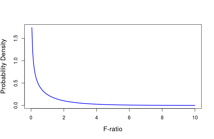
Notice that the smallest possible F-ratio is zero.
An F-ratio greater than 10 is exceedingly unlikely.
Using this distribution, the p-value is calculated as
p<10-15
Step 3: Make a decision
The p-value (p<10-15) is well below 5%
(it is so small the computer can only give an upper bound).
So we reject the null-hypothesis.
It is also important to state the estimated effect size and its uncertainty.
Some limitations...
- We can never use a p-value as evidence that H0 is true
(since a p-value assumes H0 to be true). - A large p-value (close to 1) does not give evidence in favour of H0. A large p-value indicates that the data cannot discriminate between H0 and H1.
- H0 can always be rejected given enough observations.
- A p-value tells us nothing about the effect size.
- For decisions to be robust the fitted statistical model must be a valid description of the population.
- Performing multiple hypothesis tests can be challenging (see the lesson on Errors and post-hoc tests)
Key Points
- Null-hypothesis testing compares two fitted models (models corresponding to H0 and H1)
- Null-hypothesis tests give evidence to reject the null-hypothesis
- The calculated p-value assumes H0 is true
- Report estimated effect sizes (and uncertainties) along with hypothesis test results.